Pivot Tables Explained with an Indian Sales Example
A pivot table is the fastest way to answer questions like *how much did each salesperson sell this month* or *which city gave the most orders*, from thousands of rows, without writing a single formula.
What you need first
One clean table: headings in one row, one row per sale, no blank columns, no subtotal rows inside the data. For example: Date, Salesperson, City, Product, Qty, Amount. If your data has merged cells or totals typed in the middle, fix that first, or the pivot will count the totals twice.
Build it in two minutes
1. Click any cell inside the data.
2. Insert → PivotTable → New Worksheet → OK.
3. In the field list, drag Salesperson into Rows and Amount into Values.
You now see each salesperson with their total. Drag City into Columns and the same table splits by city. Drag Product into Filters and you can look at one product at a time.
Five settings that turn it into a report
- Group dates into months: right-click any date in the pivot → Group → Months (and Years if the data runs past March).
- Show % of total: add Amount to Values a second time, right-click it → Show Values As → % of Grand Total.
- Count instead of sum: Value Field Settings → Count gives the number of orders.
- Sort: right-click a value → Sort → Largest to Smallest, so the best performer is on top.
- Refresh: a pivot does not update by itself. Right-click → Refresh after the data changes. If your data is an Excel Table (Ctrl + T), new rows are included on refresh.
Common mistakes
- Selecting only part of the data before inserting the pivot, so new rows are left out. Use an Excel Table.
- Amounts stored as text, which show as *Count of Amount* instead of *Sum*. Convert them to numbers.
- Typing over a pivot by hand. Change the data and refresh instead.
- Dates that are text. They cannot be grouped into months until they are real dates.
A monthly sales report from one pivot
Put Month in Rows, Salesperson in Columns, Amount in Values, and add a Region slicer (PivotTable Analyze → Insert Slicer). One click on a region and the whole report changes. Add a pivot chart and you have most of a monthly MIS.
Going further
Once pivots feel easy, the next steps are the Data Model (pivots across several tables), Power Query (clean the export automatically before it reaches the pivot) and dashboards with slicers. Our Advanced Excel Course covers each of these with practice data shaped like real exports.
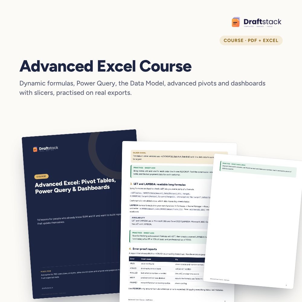 The template from this guideAdvanced Excel Course: Pivot Tables, Power Query & Dashboards
₹337
 WhatsApp
Free Monthly Budget Sheet
A printable one-page budget sheet: income, fixed bills, daily spending and savings for the month. Print it or fill it on your phone.
More guides
How to Learn Excel in 30 Days: A Day-by-Day Plan
A realistic 30-day plan to learn Excel from zero to pivot tables and dashboards, with what to practise each day and the mistakes that slow people down.
How to Collect Payments Faster from B2B Customers
Set credit limits and terms, invoice correctly, remind before the due date, log every promise, escalate politely and know when to hold orders.
How to Plan Headcount and Salary Budget for Next Year
Build a manpower budget from roles up: current staff, increments by month, phased new hires, employer costs, attrition and the year-end run-rate.